Slaying the Beast: The Bank of Canada's Ongoing Battle with Inflation

The Study In Brief

• The surge of inflation as economies recovered from the COVID lockdowns of 2020 and 2021 took central bankers and most other observers by surprise. Canada was no exception. Year-over-year CPI inflation rose from -0.4 percent at its nadir in May 2020, to a peak of 8.1 percent in June 2022 before finishing 2022 at 6.3 percent.
• In this E-Brief, we start with a short overview of the evolution of the Canadian economy and the Bank of Canada’s monetary policy since 2020 (following up on Ambler and Kronick 2021). We focus on indicators relevant to the Bank of Canada’s inflation target. Second, we analyze several different indicators of the Bank’s monetary policy stance over the post-COVID period to understand where and by how much the Bank fell behind the curve as inflation took off. In this analysis, we use a series of different Taylor rules, which predict what the Bank’s policy rate should be based on economic factors such as the gap between actual and potential output, and the gap between actual inflation and the Bank’s target, complemented by a measure of the money overhang.How much trend money growth over a period of time outpaces trend inflation, viewed against historical averages. The greater the gap, the more inflation is likely to have to stay above target to catch up. We then explore possible reasons for the Bank’s delayed tightening.
• Our analysis confirms that the Bank of Canada’s policy rate lagged behind the ideal level predicted by different variations of the basic Taylor rule. Most of the predicted values for the policy rate have now peaked or are only slightly above the current overnight rate. Alongside the closing of the gap between the trend growth rate of broad money and inflation, the evidence suggests the Bank of Canada is right to pause its tightening cycle.

The authors thank Parisa Mahboubi, Alexandre Laurin, Ted Carmichael, Pierre Duguay, David Laidler, Dave Longworth, Angelo Melino, John Murray and anonymous reviewers for helpful comments on an earlier draft. The authors retain responsibility for any errors and the views expressed.

The Canadian Macroeconomy, 2020–2022

As the COVID pandemic struck in 2020, the economy quickly took a turn for the worse. As shown in Table 1, real economic growth in the first two quarters of 2020 was negative, and the drop in the second quarter was the largest quarterly drop on record. Based on monthly data on GDP by industry, growth turned negative in March, was even more negative in April, and turned positive again in May of that year. The April decrease in particular was the steepest on record. Using the C.D. Howe Institute’s Business Cycle Council dating, this was one of the shortest recessions on record, and the deepest since the Great Depression in 1929.See Business Cycle Council (2020, 2021) for more. Based on monthly data, economic growth was negative in only two months during that recession, but it was enough to yield negative growth in each of the first two quarters of 2020.

Other goods and labour market indicators corroborate the rapidity of the GDP decline: employment fell by 28.8 percent in the second quarter of 2020, the unemployment rate reached 13.6 percent in April, and the Bank of Canada’s two measures of the output gap fell to -13.9 percent and -11.5 percent.

In response to these developments, the Bank cut its target overnight rate during March 2020 in three 50-basis-point steps. On March 27, it reached the rate’s effective lower bound of 25 basis points. On the same day, it initiated its Government of Canada Bond Purchase Program, buying $5 billion in federal debt every week. This program was initially meant to support the overall goal of stabilizing financial markets. Later, it morphed into quantitative easing (QE), which consists of buying up longer-term government bonds with the goal of keeping longer-term yields low in order to aid in the recovery of aggregate demand.

In the third quarter of 2020, the first full quarter of positive growth, GDP increased by 41.3 percent (annualized), leading to one of the fastest recoveries on record. By the last quarter of 2021 the recovery was complete, because GDP surpassed its level in the fourth quarter of 2019 (the last quarter before the recession). Employment grew by 26.9 percent in the third quarter of 2020, and reached its pre-pandemic level in October of 2021.

How did inflation evolve over this period? The pandemic recession resulted from a simultaneous decline in supply and demand. The forced shutdown of many sectors of the economy reduced supply. The temporary or permanent loss of jobs combined with a lack of spending opportunities caused a drop in demand. Initially, the drop in demand exceeded the drop in supply, explaining the dramatic drop in inflation at the beginning of the pandemic. The quarterly numbers in Table 1 mask the dramatic fall in inflation. The consumer price index (CPI) dropped by 0.58 percent from February to March 2020, an annualized inflation rate of -6.8 percent. Annualized inflation from March to April was -7.6 percent.

The federal government’s income support programs during the pandemic, plus the lack of spending opportunities, pushed the household savings rate to 28.2 percent in the second quarter of 2020. This coincided with massive increases in both narrow and broad monetary aggregates (M1++ and M2++). When the economy began re-opening, pent-up savings led the growth in demand to outstrip the growth in supply. Supply was constrained by supply-chain bottlenecks, primarily caused by lockdowns. They proved to be more persistent than the Bank of Canada (and many other analysts) anticipated, in part because of labour re-allocation away from sectors that were locked down and hard to reverse.

As the growth in demand outstripped the growth in supply, inflation soared. Monthly headline inflation increased above the 2 percent target for the first time in March 2021 (2.2 percent). It went above the upper end of the Bank’s 1-to-3 percent target range in April 2021 (3.4 percent), continued to accelerate during the rest of 2021 and early 2022, and reached 6.7 percent in March 2022 when the Bank of Canada started raising its target overnight rate from its 25 basis-point floor.

However, inflation continued higher. It peaked in June 2022 at 8.1 percent, up 1.4 percentage points from March, while the target overnight rate increased by only 1 percentage point (0.5 percent to 1.5 percent).

On the basis of these numbers, underestimating both the persistence of the economy’s supply constraints and the growth in demand seems to have led the Bank of Canada to fall behind the curve in terms of raising its policy rate to fight inflation. While the Bank was not alone among central banks in this regard – and, indeed, was first among its peers to begin tightening, and as a result the first to go on pause – it is important to delve deeper into measures that explore when and where they fell behind. Would any other indicators have given the Bank clues that inflation was coming? And where do we stand in the inflation fight at present? Our proposed measures of the appropriate monetary policy stance are designed to explore these questions in more detail.

Measuring the Stance of Monetary Policy

In this section, we start by looking at a series of simple variations on the Taylor rule that match the historical behavior of advanced central banks like the Bank of Canada, and, when followed, do well in stabilizing inflation.See Taylor (1993 and 1999), Federal Reserve Board (2018), and Federal Reserve Bank of Cleveland (2022). The Bank, like the Fed, does not mechanically follow any rule. The basic Taylor rule is a simple model describing what drives central banks to increase or decrease their policy rate (see online Appendix). From Federal Reserve Board (2018): “the Taylor rule is the best-known formula that prescribes how policymakers should set and adjust the short-term policy rate in response to the values of a few key economic variables.”

The logic of the Taylor rule is simple. The central bank’s policy rate responds positively to increases in inflation and to increases in the output gap (the difference between output and full-capacity output). The latter increases upward pressure on inflation because firms are more incentivized to raise their prices because of strong demand. Increasing the policy rate reduces demand, lowering the output gap and driving down inflation. The total response of the policy rate to inflation must be greater than one in order to increase the real interest rate, which is necessary to drive down demand.

Estimating these rules gives us a range within which the overnight rate might have been expected to fall during the COVID period to bring inflation back to target over the Bank’s 6-to-8 quarter period.Deviations from the rule don’t necessarily tell us whether monetary policy is too loose or too tight at a given moment in time. One approach that does get us to such a conclusion is to use Rowe and Tulk (2003) who ask whether deviations from the inflation target six to eight quarters ahead are positively correlated with current deviations of the overnight rate from the rule. If so, monetary policy was too loose and the Bank would have been better served following the rule more closely. We did this in past work (Ambler and Kronick 2021), but the issue for the time period we are interested in (the COVID period) is inflation’s upward march really began in March 2021 so six to eight quarters before would put us pre-COVID. We can at best look at the last few months in our sample, which do suggest a monetary policy stance that was too loose, but there are too few data points to run the Rowe and Tulk regression and say anything conclusive. The data we use – in particular output and inflation – are, of course, not available contemporaneously to the Bank of Canada at the time of policymaking. The Bank makes use of both historical data and its own forecasts/now-casts.

The Taylor rule has been a good empirical predictor of policy rate movements for different central banks (see, for example Berger and Kempa 2012). It has also been shown to be a good approximation of the optimal monetary policy in formal models of the type used by the Bank of Canada and other central banks.See for example Blake (2000). Work at the Federal ReserveSee Federal Reserve Board of Governors (2018), the Federal Reserve Bank of Cleveland (2022), and Knotek et al. (2016) for a detailed discussion. has gone further, arguing that while the basic Taylor rule might be the best-known model for how policymakers ought to set and adjust their policy rate, many alternatives have been developed, and by examining these alternatives, we get a better understanding of the possible range of policy rate outcomes. As an example, one of these alternatives includes a rule that adjusts for crisis periods where the overnight rate hits its effective lower bound (ELB) and more monetary stimulus is needed.

We start this section by calculating and analyzing what the range of Taylor rules tell us about the Bank of Canada’s response during the crisis.

We complement this Taylor rule work with analysis that focuses more on monetary aggregates. Until the early 1980s, many economists observed a tight positive correlation between monetary aggregates and inflation in both the short and long term. However, this relationship deteriorated in the mid-1980s, and most central bankers today pay little attention to monetary aggregates. As shown in Ambler and Kronick (2022), this positive correlation between money growth and inflation returns when inflation is unanchored from its target – a situation we find ourselves in today – and the former can help predict the latter as well.When a central bank is hitting its target on average, then Rowe and Yetman (2002) and Otto and Voss (2014) show theoretically and empirically that observed deviations of inflation from target must be unpredictable with respect to an appropriately defined information set, which would include money growth. These results are consistent with others, including recent work from Borio et al. (2023) at the Bank for International Settlements (BIS) who find, among other things, that “the strength of the link between money growth and inflation depends on the inflation regime: it is one-to-one when inflation is high and virtually non-existent when it is low.”

Looking at money is also helpful when unconventional monetary policy like quantitative easing (and quantitative tightening) has occurred, especially alongside the fiscal stimulus we have seen over the last few years. In such cases, we have a textbook case of helicopter money fueling pent-up demand that will show itself in monetary aggregates.

Taylor Rules

We look at seven Taylor rules and create a range and a median of the rules’ results to compare against the actual overnight rate. We look at the whole period from January 1996 to December 2022. Full descriptions of the rules and variables are available in online Appendix A. With the exception of the core inflation rule, we use headline inflation for the others.All variables are available monthly except the OECD inflation forecast data and the Bank of Canada’s output gap data, which are available quarterly. For these two variables, we interpolate them to make them monthly. The seven rules (with short descriptions) are as follows:

1. The basic Taylor rule, which puts a coefficient of 0.5 on inflation’s deviation from target and the output gap;
2. A balanced-approach rule, which puts a higher weight (1) on the output gap term;
3. A core inflation rule, which uses core inflation instead of headline inflation and follows the balanced-approach rule;
4. A forward-looking rule, which uses the basic Taylor rule but instead of using contemporaneous inflation relative to target, uses a forecast of inflation some periods ahead;
5. An inertial rule, which uses the balanced-approach rule but spreads the interest rate adjustments over time to reduce volatility;
6. An ELB-adjusted rule, which uses the balanced approach rule but sets the rate at the ELB whenever the rule prescribes a rate below – to compensate, it keeps the overnight rate below the ELB for a period of time after; and
7. A rule based on Choudhri and Schembri (2013), who estimate the coefficients on inflation’s deviation from target and the output gap for a given period – less than the full sample – then use those estimates to generate out-of-sample predicted values to compare to what the Bank of Canada actually did.

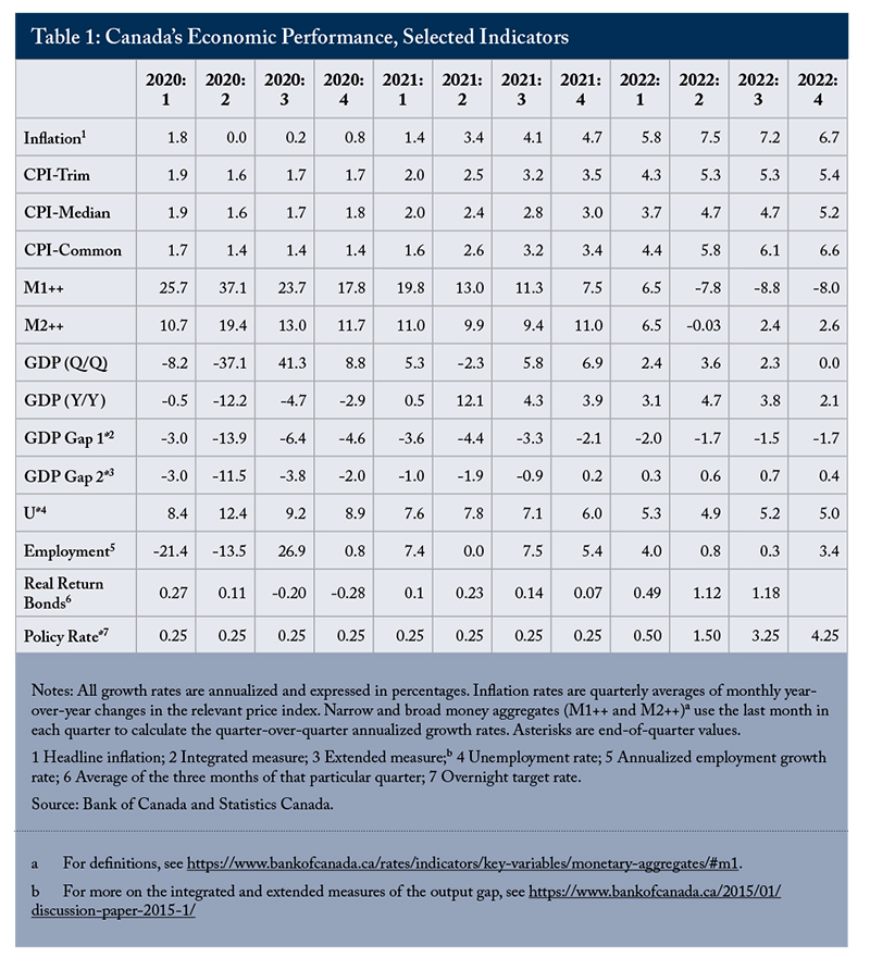
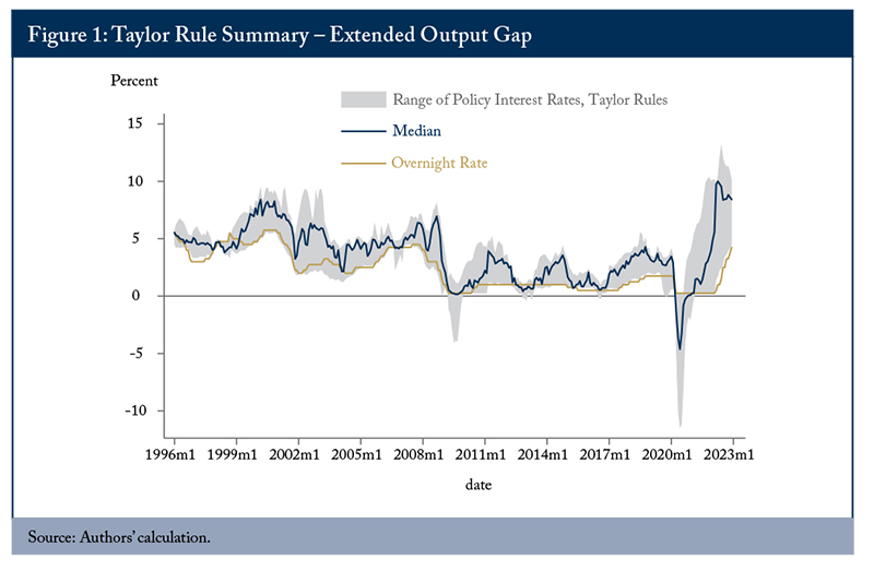
Figures 1 and 2 show the range of policy interest rates given by the different versions of the Taylor rule (in grey) along with the median of these rules and the actual Overnight Rate Target (ONR). The extended output gap is used to generate the predicted policy rate in Figure 1, while the integrated output gap is used in Figure 2.

The target overnight rate remains within the grey band of possible predicted values more often than not over the sample period. However, it appears that using the median of the rules, the Bank should have started lifting off the ELB to combat rising inflation beginning in February 2021 for the extended output gap measure, and July 2021 for the integrated output gap measure. Inflation was only 1.1 percent in February 2021, but the next month jumped to 2.2 percent, and by July 2021 was 3.7 percent. This reinforces the idea that the Bank of Canada, like most central banks, fell behind the curve in fighting inflation.The lower end of the range during that first half of 2021 was supported by the core inflation rule, the ELB-adjusted rule and the inertial rule. As robustness, we reran these rules replacing the output gap with the difference between unemployment and its natural rate, which also allows us to go to February 2023. The results do not change (available from the authors upon request). Liftoff from the ELB would have been March 2021 under this setup – the month headline inflation first jumped above the 2 percent target.

Money Growth and Inflation

Might other measures have helped the Bank of Canada (and other central banks) anticipate that inflation was coming even if the period after the Great Financial Crisis (GFC) had seen most countries fail to hit their central bank’s inflation target? Yes – money.

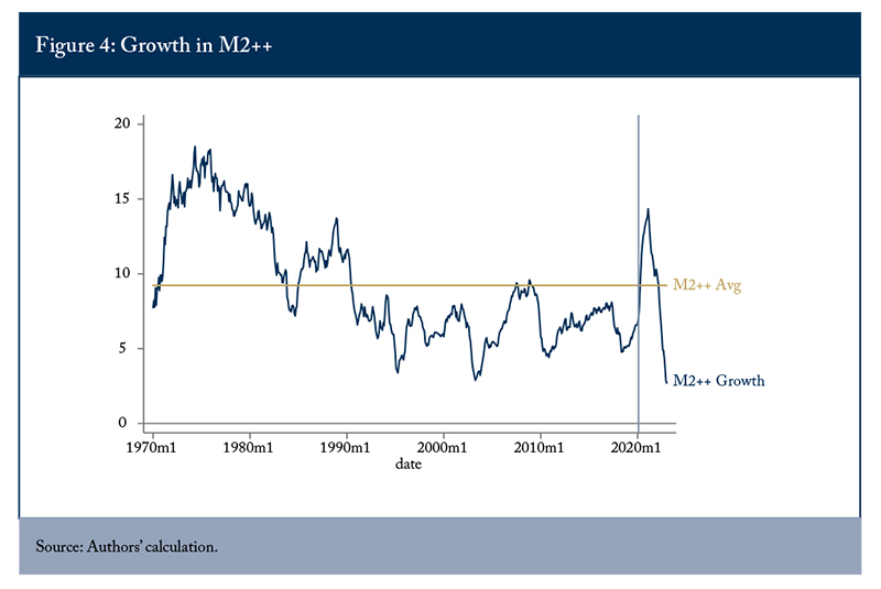
As a result of massive pandemic supports from both the Bank of Canada in the form of quantitative easing, and governments in different forms of fiscal stimulus, money growth spiked to levels not seen on record in the case of narrow money (M1++) and not since before inflation-targeting began in the early 1990s for broad money (M2++) (Figures 3 and 4). The likelihood of this money growth having an impact on inflation was exacerbated by the fact that that money had no place to be spent in the early days of the pandemic when lockdowns shuttered businesses.

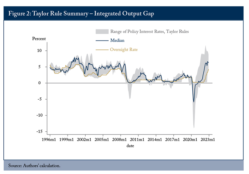
As things opened up, this money overhang combined with supply-chain snarls caused more money to chase fewer goods leading to above-target inflation. As we mentioned above, while money lost favour with central bankers as it lost predictive power for inflation, we showed in Ambler and Kronick (2022) – as did others like Borio (2023) – that this predictive power returns when inflation becomes unanchored form its target like it is today.

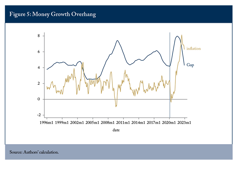
One way of looking at how money growth might help predict future inflation – even before it becomes unanchored – is to look at long-run trends of each. If growth in trend money over a certain period outpaces trend inflation, an overhang exists and we would expect inflation to have to catch up with further monetary policy tightening. Following our past work, Ambler and Kronick (2022), we use what’s called a Hodrick-Prescott (HP) filter to decompose money growth (using M2++ as our preferred broad money aggregate) and inflation data “into a trend (long-run or structural) component and a cyclical component (short-run, subject to short-lived shocks)” (ibid.). We use these as measures of trend growth rates and take an increase in the difference between trend money growth and trend inflation as a measure of money growth “overhang.” One element we do differently here in updating this past work is instead of looking at the gap using all historical data, we evaluate how the gap in the two trend variables evolves over time using the data policymakers would have had in real time. There is always a positive difference between trend money growth and trend inflation and what we want to see is whether that difference grows or shrinks over time using only the most recent data policymakers have when making monetary policy decisions. We graph this gap against inflation (Figure 5). As we see, the gap shot up right when the pandemic hit (as signaled by the grey vertical bar), and inflation soon followed. From Figure 4, we can tell that the spike in the gap was due to a spike in money growth (compared to the spike in the gap during the GFC, which was not). Similarly, as the gap came back down with monetary policy tightening, inflation has started to as well. Since the gap essentially sits where it was when the pandemic began, we argue that no more tightening is likely necessary as inflation will continue to shrink until it is back in line with where it was pre-pandemic.

Discussion of Results – Why Central Banks Including the Bank of Canada Fell Behind the Curve

The results of the previous section show a complete consensus among the Taylor rules that the Bank was right to drop the overnight rate to its ELB at the beginning of the pandemic. In fact, many of them suggest the Bank should have gone negative. However, the Bank views 25 basis points as the effective lower bound for its policy rate, so it did not reduce its policy rate below zero.Some central banks (the European Central Bank, the Swiss National Bank and Sweden’s Riksbank) have operated with policy rates below zero. We noted that as it reduced its policy rate to 25 basis points, the Bank began purchasing large quantities of financial assets. The initial intention was to calm financial markets, but it quickly morphed into a policy of quantitative easing (QE).

The goal of QE is to support aggregate demand by driving up the price of bonds with longer terms to maturity, thereby driving down their yields.The effectiveness of QE has been disputed (see for example Thornton 2015): it is difficult to drive down long-term yields when yields are already low across the yield curve. The Bank supplemented its QE program by providing forward guidance, promising to keep its policy rate low for an extended period of time, also in order to boost aggregate demand. Its July 2020 interest rate announcement (Bank of Canada 2020) noted, “The Governing Council will hold the policy interest rate at the effective lower bound until economic slack is absorbed so that the 2 percent inflation target is sustainably achieved.”

As just discussed, using the median of our Taylor rules recommended a liftoff of the policy rate from its lower bound somewhere between February and July 2021. The Bank did end its QE program in October 2021, in advance of other central banks. However, it did not remove its forward guidance until January 2022, and did not begin raising its policy rate until March of that year. This confirms our hypothesis stated above that the Bank fell behind the curve in raising its policy rate. We think five factors explain this.

1. The Bank (along with other central banks and most professional forecasters) underestimated the persistence of supply chain bottlenecks.
2. The unusual nature of the economic shocks that led to the pandemic recession (forced shutdowns of many sectors of the economy plus the fall in aggregate demand resulting from a lack of many spending opportunities during lockdowns) meant that it was difficult to predict the size of the output gap. Table 1 shows that the two traditional measures the Bank uses were both negative through the third quarter of 2021.
3. Headline inflation measures the average of (annualized) monthly changes in the consumer price index (CPI) over the preceding twelve months. By construction, this measure has a high degree of persistence. Headline inflation moved above the 2 percent target for the first time in March 2021. This number included changes in the CPI from early in 2020, when it was still decreasing. This means that prices were increasing more rapidly in 2021 than the headline inflation numbers indicated.
4. The Bank’s forward guidance meant promising to keep its policy rate lower for longer. The promise was conditional on the persistence of excess productive capacity in the economy but, as we note in our second point, measuring this became difficult due to the unusual nature of the pandemic shocks, which led to the persistence of the supply bottlenecks.
5. Lastly, with all that going on, the continued belief that monetary aggregates had lost relevance in predicting future inflation. The evidence is increasingly clear that the link returns when inflation becomes unanchored, but we would take this a step further, as we showed above, that large shocks to money – such that they increase money’s long-run trend growth – act as leading indicators for future inflation.

Conclusions and Policy Recommendations

Our analyses of several different versions of the Taylor rule confirm that the Bank of Canada’s policy rate lagged behind its expected values during the fight against well-above-target inflation. To some extent, it still does today, however, most of the predicted values have peaked or are only slightly above the current overnight rate. With the gap between the trend growth rate of broad money and inflation now closed, the evidence suggests that the Bank’s rate tightening cycle should be at its end. Headline inflation, which peaked in June 2022, should continue to decelerate, aided by falling trend money growth, and this will lead to a convergence between the policy rates recommended by the different simple monetary policy rules analyzed here and the Bank’s target overnight rate. In other words, the Bank of Canada is right to pause its tightening cycle. There are many lessons for the Bank of Canada and other central banks from this episode. They include: (i) the challenges in estimating the output gap in crisis periods exacerbated by huge supply chain bottlenecks, and the consequences for the appropriateness of forward guidance; (ii) the dangers of using year-over-year CPI when there have been large swings in prices, and the importance, then, of complementing the analysis with a month-over-month or other shorter duration measure; and lastly, (iii) the importance of money growth when it experiences large shocks, or changes, as a leading indicator of changes in inflation.

References

Ambler, Steve, and Jeremy Kronick. 2020. “Canadian Monetary Policy in the Time of COVID-19.” E-Brief 307. Toronto: C.D. Howe Institute.

___________. 2021. For the Record: Assessing the Monetary Policy Stance of the Bank of Canada. Commentary 588. Toronto: C.D. Howe Institute.

___________.2022. Money Talks: The Old, New Tool for Predicting Inflation. Commentary 623. Toronto: C.D. Howe Institute.

Bank of Canada. 2020. “Bank of Canada will maintain current level of policy rate until inflation objective is achieved, continues program of quantitative easing.” Ottawa: Bank of Canada, July 15.

Berger, Tino, and Bernd Kempa.2012. “Taylor Rules and the Canadian–US Equilibrium Exchange Rate.” Journal of International Money and Finance 31: 1060–1075.

Blake, Andrew. 2000. “Optimality and Taylor Rules.” National Institute Economic Review 174: 80–91.

Borio, Claudio, Boris Hofmann, and Egon Zakrajsek.2023. “Does Money Growth Help Explain the Recent Inflation Surge?” BIS Bulletin No 67. January.

Business Cycle Council. 2020. “Canada Entered Recession in First Quarter of 2020.” Communiqué. Toronto: C.D. Howe Institute, May 1.

Business Cycle Council. 2021. “C.D. Howe Business Cycle Council Declares an End to the COVID-19 Recession.” Communiqué. Toronto: C.D. Howe Institute, August 24.

Choudhri, Ehsan, and Lawrence Schembri. 2013. “A Tale of Two Countries and Two Booms, Canada and the United States in the 1920s and the 2000s: The Roles of Monetary and Financial Stability Policies.” Working Paper 44_13, Rimini Centre for Economic Analysis. Accessed at: http://www.rcea.org/RePEc/pdf/wp44_13.pdf

Federal Reserve Bank of Cleveland. 2022. “Monetary Policy Rules.” Accessed at:
https://www.clevelandfed.org/our-research/indicators-and-data/simple-monetary-policy-rules/

Federal Reserve Board of Governors. 2018. “Policy Rules and How Policymakers Use Them.” Accessed at: https://www.federalreserve.gov/monetarypolicy/policy-rules-and-how-policymakers-use-them.htm

Holston, K., T. Laubach, and J. Williams. 2017. “Measuring the Natural Rate of Interest: International Trends and Determinants,” Journal of International Economics 108, supplement 1: S39–S75. May.

International Monetary Fund. 2022. “World Economic Outlook.” Various issues. Accessed at:
https://www.imf.org/en/Publications/WEO

Knotek, Edward, Randal Verbrugge, Christian Garciga, Caitlin Treanor, and Saeed Zaman. 2016. “Federal Funds Rates Based on Seven Simple Monetary Policy Rules.” Economic Commentary 2016-07, Federal Reserve Bank of Cleveland. Accessed at:
https://www.clevelandfed.org/newsroom-and-events/publications/economic-commentary/2016-economic-commentaries/ec-201607-federal-funds-rates-from-simple-policy-rules.aspx

Otto, Glenn, and Graham Voss. 2014. “Flexible Inflation Forecast Targeting: Evidence from Canada.” Canadian Journal of Economics. July. Accessed at: https://doi.org/10.1111/caje.12083

Pichette, Lise, Pierre St-Amant, Ben Tomlin, and Karine Anoma. 2015. “Measuring Potential Output at the Bank of Canada: The Extended Multivariate Filter and the Integrated Framework.” Bank of Canada Discussion Paper 2015-1. January.

Rowe, Nicholas, and David Tulk. 2003. “A Simple Test of Simple Rules: Can They Improve How Monetary Policy Is Implemented with Inflation Targets?” Working Paper 2003–31. Ottawa: Bank of Canada. Accessed at: https://www.bankofcanada.ca/2003/10/working-paper-2003-31/.

Rowe, Nicholas, and James Yetman. 2002. “Identifying a Policy-Makers’ Target: An Application to the Bank of Canada.” Canadian Journal of Economics 35:239–256.

Taylor, John.1993. “Discretion versus Policy Rules in Practice.” Carnegie-Rochester Conference Series on Public Policy 39: 195–214.

Taylor, John.1999. “A Historical Analysis of Monetary Policy Rules.” Monetary Policy Rules. Chicago: University of Chicago Press, 319-341.

Thornton, Daniel. 2015. “Requiem for QE.” Policy Analysis 783, Washington DC, Cato Institute.

Online Appendix

The Taylor Rule and Its Variations

Basic Taylor Rule

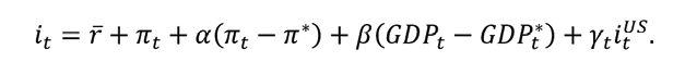
The basic Taylor ruleSee Taylor (1993). says that the central bank’s policy rate depends on a constant long-term neutral rate, on the difference between current inflation and the inflation target, and on the difference between the current level of GDP and its full-employment level (the output gap). It can be written as follows.

Here, it is the central bank’s policy interest rate (the target overnight rate in the case of the Bank of Canada),  is the long-term real natural rate of interest,This is assumed to be constant in the simplest form of the rule. πt is the current inflation rate, π* is the inflation target, GDPt is the current level of real GDP,In practice, this will be the best now-cast of GDP on the basis of all currently-available information. GDPt* is the estimated level of full-capacity output, and α and β are positive constants or parameters chosen so that the central bank’s choice of its policy rate is approximately optimal.

Taylor (1993) initially sets the real natural rate equal to 2.0, the inflation target to 2.0 (which also of course coincides with the Bank of Canada’s target), and α = β = 0.5.This means that the policy rate reacts more than one-for-one to changes in the inflation rate. This is necessary for the real interest rate to vary in the same direction as the inflation rate and is known as the Taylor principle. If it is not satisfied, higher inflation will lead to a lower real interest rate, which will boost aggregate demand and cause inflation to increase even more, leading to instability.

We use a slight variation on the original Taylor (1993) in that we allow the real neutral rateThe rate at which the economy is operating at its full potential with inflation sustainably at its target. to vary over time. We use real return bonds as our measure of the real neutral rate for this and for the other Fed rules.Holston et al. (2017) estimate a real neutral rate for Canada (among other countries). However, it ends in the second quarter of 2020. We also use both output gapWe use the Extended Multivariate Filter and the Integrated Framework output gap measures from the Bank of Canada. See Pichette at al. (2015) for more details on each measure. measures from the Bank of Canada.

Balanced Approach

The balanced-approach rule is identical to the simple Taylor rule except that the coefficient on the output gap – 1 – is double that of the inflation coefficient. This is done to ensure the Bank responds more forcefully to the output gap than to inflation deviations from target.

Core Inflation Rule

The core inflation rule is simply the balanced approach rule where headline inflation is replaced with core inflation. For core inflation we use one of the Bank of Canada’s preferred measures, CPI-Median, which from the Bank’s site is “a measure of core inflation corresponding to the price change located at the 50th percentile (in terms of CPI basket weights) of the distribution of price changes in a given month.”

Forward-looking Rule

The forward-looking rule is also similar to the basic Taylor rule except that instead of using contemporaneous inflation relative to target, it uses a forecast of inflation some periods ahead. The idea here is that since monetary policy works with a lag, what matters is not inflation today but inflation at some future moment in time. We use inflation forecast data from the OECD.See https://data.oecd.org/price/inflation-forecast.htm for more data on the OECD inflation forecast measure. The measure is available quarterly and we interpolate to make monthly. Following the Federal Reserve Bank of Cleveland, the formula is

Inertial Rule

The inertial rule takes the balanced-approach rule but acknowledges that the central bank may not want to increase rates immediately, preferring to spread out the adjustments over time. The idea behind this more gradual approach is it decreases short-term interest rate volatility. We use the inertia coefficient from the Federal Reserve Board. The formula is

Effective Lower Bound-Adjusted Rule

An economy that requires additional stimulus may run up against the constraint that the overnight rate cannot drop any further. Taylor rules as we’ve described so far would have trouble reconciling this fact, suggesting the central bank run significantly negative overnight rates when it cannot. The ELB-adjusted rule would tell the central bank to keep it at the ELB when the balanced approach suggests a negative rate. The ELB-adjusted rule would then prescribe a period of time where the overnight rate stays at the ELB despite the balanced-approach suggesting it was time to raise it. In formal terms:

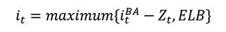
where itBA is the overnight rate suggested by the balanced approach rule, Zt represents “the cumulative shortfall in monetary stimulus that occurs because short-term interest rates cannot be reduced below the ELB” (Federal Reserve Board 2022). This shortfall must then be shrunk to zero before the overnight rate comes off the ELB.

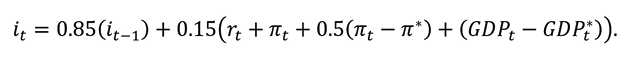
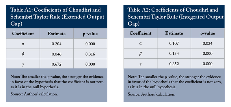
Choudhri and Schembri Taylor Rule

Choudhri and Schembri (2013) modify the simple Taylor rule (with a fixed real neutral rate) for Canada by including the US policy rate. They also use regression analysis to estimate (rather than simply choosing values thought to be approximately optimal) the values of the α and β coefficients using quarterly data from 1990:Q1 to 2001:Q4, and generate predicted values for the target overnight rate over the 2002–2007 period. We estimate with data from January 1996 until February 2020 – right before the pandemic – and then generate predicted values from March 2020 to December 2022.The great financial crisis (GFC) period was included without adjustment in the estimation as the predicted values during this timeframe were not significantly below the ELB – indeed, they were never negative. The formula is:

The coefficients for α, β, and γ are found in Table A1 alongside their p-values (p-values below 0.10 are significant at more than 90 percent).