Predicting Financial Crises: The Search for the Most Telling Red Flag in the Economy

Study in Brief

Canada is often cited as having worryingly high household debt-to-GDP and debt-to-disposable-income ratios, but the assets and net worth of Canadian households have grown more quickly than their debt.

Using a new financial vulnerabilities barometer, we show that the inclusion of household debt servicing considerably improves the barometer’s ability to track financial vulnerability, particularly in advance of recessions. In contrast to the Bank of Canada’s financial vulnerability barometer, our index declines sharply after the Great Recession and indicates that financial risks are currently quite low. By focusing on debt servicing (the debt-service-to-disposable-income ratio) rather than debt, the barometer appears to yield fewer false positives than the Bank of Canada’s barometer.

Further empirical analysis indicates that debt servicing is an improvement over traditional credit measures in predicting future economic growth and financial crises. We show that the relationship between debt servicing and both financial crises and economic growth is statistically significant. More specifically, we find that increases in new borrowing lead initially to a mild increase in economic activity and a significant reduction in the probability of financial crises, but they subsequently lead to a gradual increase in households’ debt service burden (the sum of principal and interest payments on their outstanding debts), expressed as a ratio of disposable income, which has a significantly negative impact on economic activity and a significantly positive impact on the probability of financial crises.

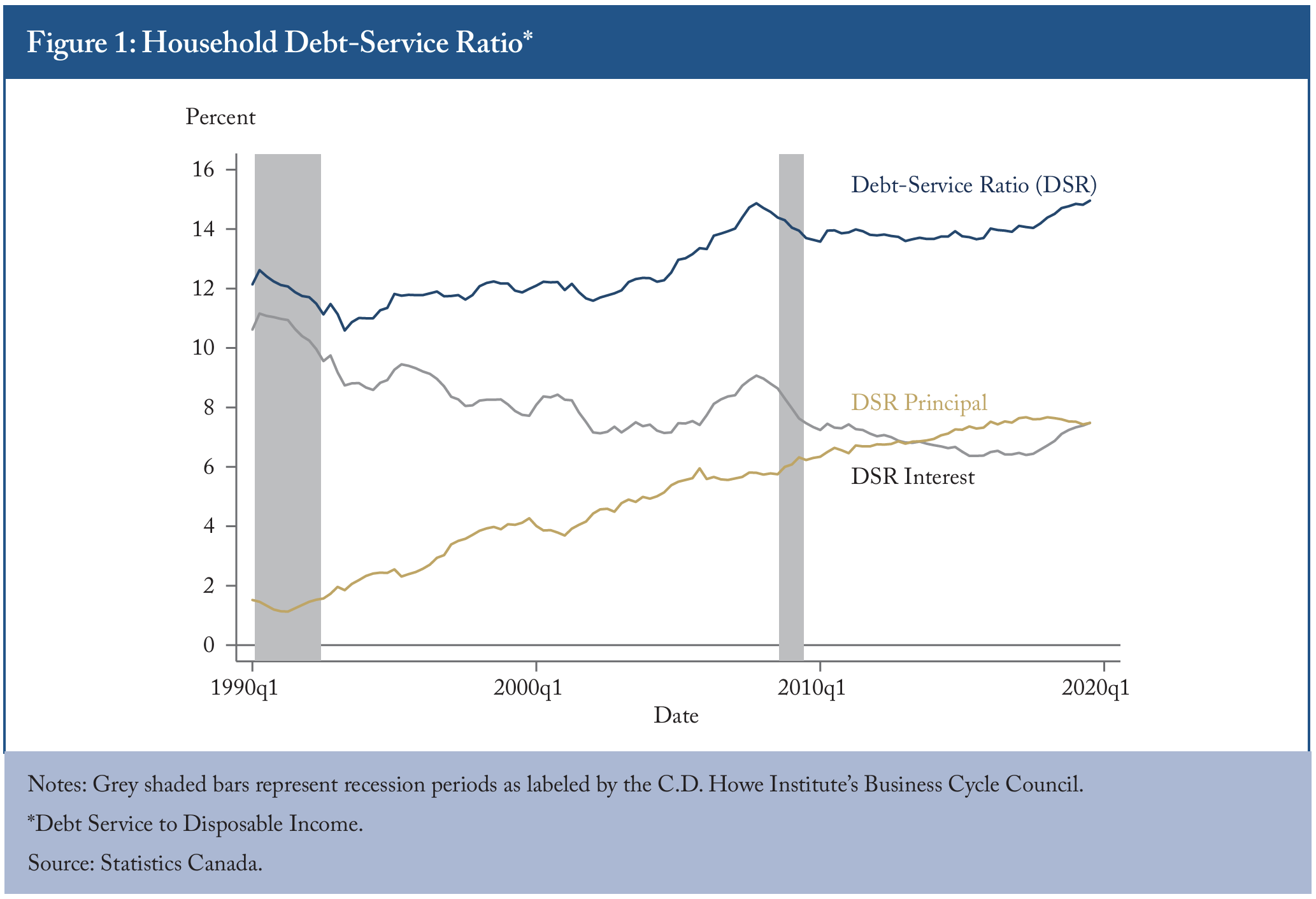
Focusing on debt servicing provides a potential clue as to why we have not seen the type of market correction that has been repeatedly predicted for the Canadian housing market – namely, the fact that over the last 25 years the debt-service-to-disposable-income ratio has largely been flat, except for a mild recent increase, and (not coincidentally) an increase before the 2008 financial crisis.

Our findings have policy implications for both the conduct of monetary policy and financial sector regulators. An immediate policy conclusion is that empirical models of financial system vulnerabilities should put more weight on the evolution of debt-service ratios and other indicators related to debt servicing. Furthermore, if financial stability is taken into consideration in the setting of monetary policy, central banks must be concerned with the trade-off between the short-run positive effects of increased borrowing on output and inflation and the potentially negative long-run effects that work their way through the debt-service channel.

Lastly, regulators concerned with the housing market and overall financial stability should look beyond traditional credit-to-GDP measures, which were always going to increase in a low interest rate environment, and closely monitor the behaviour of debt servicing.

Introduction

For much of the past decade, Canadians have heard that their debt levels were unsustainable, and that a day of reckoning was fast approaching in this respect.

Against this backdrop, new data can sound troubling. For example, the Office of the Superintendent of Bankruptcy (OSB) recently reported that insolvencies by Canadian consumers were up 8.9 percent over a 12-month period ending in November 2019, compared to the 12-month period ending in November 2018.¹1 See https://www.ic.gc.ca/eic/site/bsf-osb.nsf/eng/br04178.html. But a little context is needed.

The data also show that Canadians’ net worth has never been higher. Before the financial crisis, household net worth was a little over 7 times disposable income. It dipped during the financial crisis, bottoming out at 6.25 times disposable income. However, since then, with low interest rates boosting housing prices, net worth has been on a mostly continuous upward trend, and has been between 8.5 and 9 times disposable income since the second quarter of 2016 (in the third quarter of 2019 net worth was 8.7 times disposable income).

Moreover, while household debt to GDP has increased from 75 percent in 2007 to approximately 100 percent today, household debt to net worth has remained almost identical at around 20 percent.²2 Data from Statistics Canada 38-10-0235-01. See Ambler, Kronick and Omran (2019) for more. Also, Congdon (2017) notes that the OECD and the BIS have been ringing similar alarm bells about debt levels around the world while net assets have been increasing. “The historical experience is that assets increase by amounts so much larger than debt that the netwealth-to-income ratio and the debt-to-income ratio can and usually do rise together!” The stability of this ratio suggests (and this is confirmed by the data) that household debt and net worth move in near lock step.³3 The dip in both net worth and debt during the financial crisis reflects the deleveraging that often occurs during financial crises. See Taylor (2015) for a broad survey. From this, one can infer that increasing debt is not necessarily a red flag signaling financial difficulties, just as increasing net worth is not necessarily a green flag.

Unfortunately, the OSB data do not make a distinction between (i) defaults due to true insolvency (where net worth is negative) and (ii) defaults from illiquidity, which involves failing to meet debt payments due to the difficulty of selling one’s assets. The only distinction in the OSB data is between bankruptcies and consumer proposals, an alternative to bankruptcy where the lender and borrower strike a deal under which the latter pays back a portion of their debt over the ensuing five years (and, critically, does not have to sell their house). For the 12-month period ending November 2019, consumer proposals increased 17.4 percent while bankruptcies decreased 1.9 percent. With stable debt to net worth, and with two-thirds of Canadian households owning homes, it could be that the bulk of these consumer proposals are a result of illiquidity problems. If true, households’ debt-service burden (the sum of principal and interest payments by households on their outstanding debts) expressed as a ratio of disposable income should be critical in determining the health of household balance sheets, and thus an important predictor of defaults.

The Bank of Canada maintains a financial vulnerability barometer to help guide its monetary policy. However, it omits debt servicing. In this Commentary, we construct a modified barometer of financial vulnerabilities that uses Canadian households’ debt-service burden as a key component. We show that the barometer does a good job of tracking major recessions and periods of elevated financial stress. Including debt servicing considerably improves the barometer’s ability to track financial vulnerability, particularly in advance of recessions. In contrast to the Bank of Canada’s financial vulnerability barometer, our index declines sharply after the Great Recession and indicates that financial risks are currently quite low. By focusing on debt servicing rather than debt, the barometer appears to yield fewer false positives than the Bank of Canada’s barometer.

We also show that the relationship between debt servicing and both financial crises and economic growth is statistically significant. More specifically, we find that increases in new borrowing lead initially to a mild increase in economic activity and a significant reduction in the probability of financial crises, but they subsequently lead to a gradual increase in debt servicing, which has a significantly negative impact on economic activity and a significantly positive impact on the probability of financial crises. Our results suggest that “stock” variables, which measure a fixed amount at a moment in time, such as debt and credit levels, do not tell a complete story of the financial risks that are building in the economy.⁴4 The same applies to “stock to flow” variables, where a flow variable is measured over a period of time. Examples are debt/ GDP and debt/income ratios.

This is particularly true during a period of declining interest rates that has encouraged higher levels of borrowing relative to income.

Focusing on debt servicing provides a potential clue as to why we have not seen the type of market correction that has been repeatedly predicted for the Canadian housing market – namely, the fact that over the last 25 years the debt-service-todisposable-income ratio (hereafter, debt-service ratio) has largely been flat, except for a mild recent increase, and (not coincidentally) an increase before the 2008 financial crisis.

Our findings have policy implications for both the conduct of monetary policy and financial sector regulators. An immediate policy conclusion is that empirical models of financial system vulnerabilities should put more weight on the evolution of debtservice ratios⁵5 While we focus on the household debt service ratio, other similar ratios could be calculated for businesses, for example. and other indicators related to debt servicing.⁶6 Some recent work on the importance of debt servicing has been done at policy institutions. See Aldasoro, Borio and Drehmann (2018), Allen et al. (2017) and Bilyk, Ueberfeldt and Xu (2017). While certainly a start, more work needs to be done. Furthermore, if financial stability is taken into consideration in the setting of monetary policy, central banks must be concerned with the tradeoff between short-run positive effects of increased borrowing on output and inflation and potentially negative long-run effects that work their way through the debt-service channel. Financial sector regulators should look beyond traditional creditto-GDP measures, which were destined to increase in a low interest rate environment at any rate, and closely monitor the behavior of debt servicing. This will result in a more accurate risk assessment.

The Evolution of Debt Servicing

As shown in Figure 1, the debt-service ratio of Canadian households has been quite stable over our entire sample period, except for a mild recent increase, and, critically, in the run-up to the financial crisis. The stability largely comes from increases in principal, offset by decreases in interest rates. The figure indicates that increases in the debtservice ratio may help to predict financial stress associated with recessions, in particular the financial crisis and Great Recession of 2007-08.

While debt servicing data are not available before 1990, it is possible to generate an estimated version of debt servicing going further back in time (see Drehmann and Juselius 2012 for details how). Figure 2 backdates debt servicing to 1980. The estimated debt-service ratio seems to have peaked in advance of the early 1980s recession, as well as a sharp increase prior to the early 1990s recession. This reinforces the idea that changes in this variable may help predict financial stress.⁷7 As a result of the backdating methodology, estimated data pre-1990 were scaled down to align with actual post-1990 data. The correlation between actual post-1990 data and estimated post-1990 data if we were to extend the backdating methodology forward is very high (above 0.9).

A New Financial Vulnerability Index

The Bank of Canada (Duprey and Roberts 2017)⁸8 See also Pasricha et al. (2013). has developed a financial stability vulnerabilities barometer, which aggregates together indicators from the following four sectors: banking, corporate, household, and housing. In this section, given the correlation between debt servicing and previous recessions, we compare the evolution of the Bank’s financial stability barometer with one that incorporates indicators based on debt servicing.

Duprey and Roberts choose indicator variables on the basis of their ability to predict periods of financial stress within 24 months.⁹9 The methodology comes from the machine learning literature. In addition to Duprey and Roberts (2017), see also Fawcett (2006), Flach (2010), Swets et al. (2000) and van Erkel and Pattynama (1998). Following Duprey and Roberts, we use their dates for periods of financial stress defined (page 5) as “events where a financial stress index is two standard deviations above its trailing 10-year moving average.” A minimal criterion for selection is that a variable predicts periods of financial stress better than a coin flip. The methodology also involves the selection of threshold levels for the variables (only values above the threshold levels are predictors of financial stress) and a way of weighting the different indicators in order to construct an index. 

Because financial stress episodes are rare in individual countries, we follow Drehmann and Juselius (2014) and look at international crisis periods across a panel of countries including Canada over the 1990:Q1–2019:Q3 period. The exact dates can be found in Drehmann and Juselius. We add to this list the oil price shock and economic slowdown in 2015:Q1. These financial periods correspond to the following events:

1. The recession of the early 1990s;
2. The Mexican crisis (1994–1995);
3. The Asian crisis (1997–1998);
4. The Russian debt default (1998);
5. The Long-Term Capital Management collapse (1998);
6. The sub-prime crisis, financial crisis and Great Recession (2007–2008);
7. The aftermath of the oil price collapse (early 2015).

We simplify the Duprey-Roberts measure in a variety of ways, and focus on the additional valueadded of incorporating debt servicing. Rather than using a panel of countries to calculate threshold values, we use our own made-in-Canada measures.

We do not use all variables across sectors from Duprey and Roberts. Instead, we focus on the two indicators in each of their four sectors with the best predictive power, excluding those that conflate stock and flow variables (for example debt-to-GDP ratios). Our variables are primarily deviations from one-sided trends (calculated using only backwardlooking data). This means that they are calculated using the same information that would be available to a regulator at a particular point in time.¹⁰10 We use a one-sided Hodrick-Prescott filter. See Drehmann and Yetman (2018). A two-sided deviation from trend would include both backward and forward-looking data: the latter would obviously not be available to regulators at a particular moment in time. This exercise yields the following variables as having the best predictive power of a financial stress episode:

1. the deviation from trend of the ratio of household debt to disposable income;
2. the deviation from trend of the ratio of household debt to GDP;
3. the ratio of housing price to rent;
4. the deviation from trend of the ratio of housing price to rent;
5. the year-over-year growth rate of the ratio of non-financial corporate debt to GDP;
6. the deviation from trend of the ratio of nonfinancial corporate debt to GDP;
7. the year-over-year growth rate of the ratio of financial institution debt to GDP;
8. the deviation from trend of the ratio of financial institution debt to GDP.

We drop the ratio of housing price to rent (though keep the one-sided deviation from trend of the ratio of housing price to rent) from the sample since (unlike for Duprey and Roberts in their crosssection of countries analysis) it has low predictive power for Canada. For the debt-service ratio, we find that the deviation from trend has robust predictive power, so we add this variable to our list.

Our resulting vulnerabilities barometer is shown in Figure 3. The vertical grey bars are Canadian recessions and the vertical yellow bars represent other international financial stress episodes.¹¹11 As in Duprey and Roberts (2017) we restrict the vulnerabilities barometer to be greater than or equal to zero.

The barometer does a good job of tracking major recessions (grey bands) as well as other periods of elevated financial stress (yellow bars). Debt servicing (in dark grey) also appears to have significant value added, especially in advance of recessionary periods.

At no point since the financial crisis does the barometer reach the level of vulnerability seen before the financial crisis. (The barometer does pick up the aftermath of the oil price shock in early 2015, but unfortunately does not give much advance warning.)

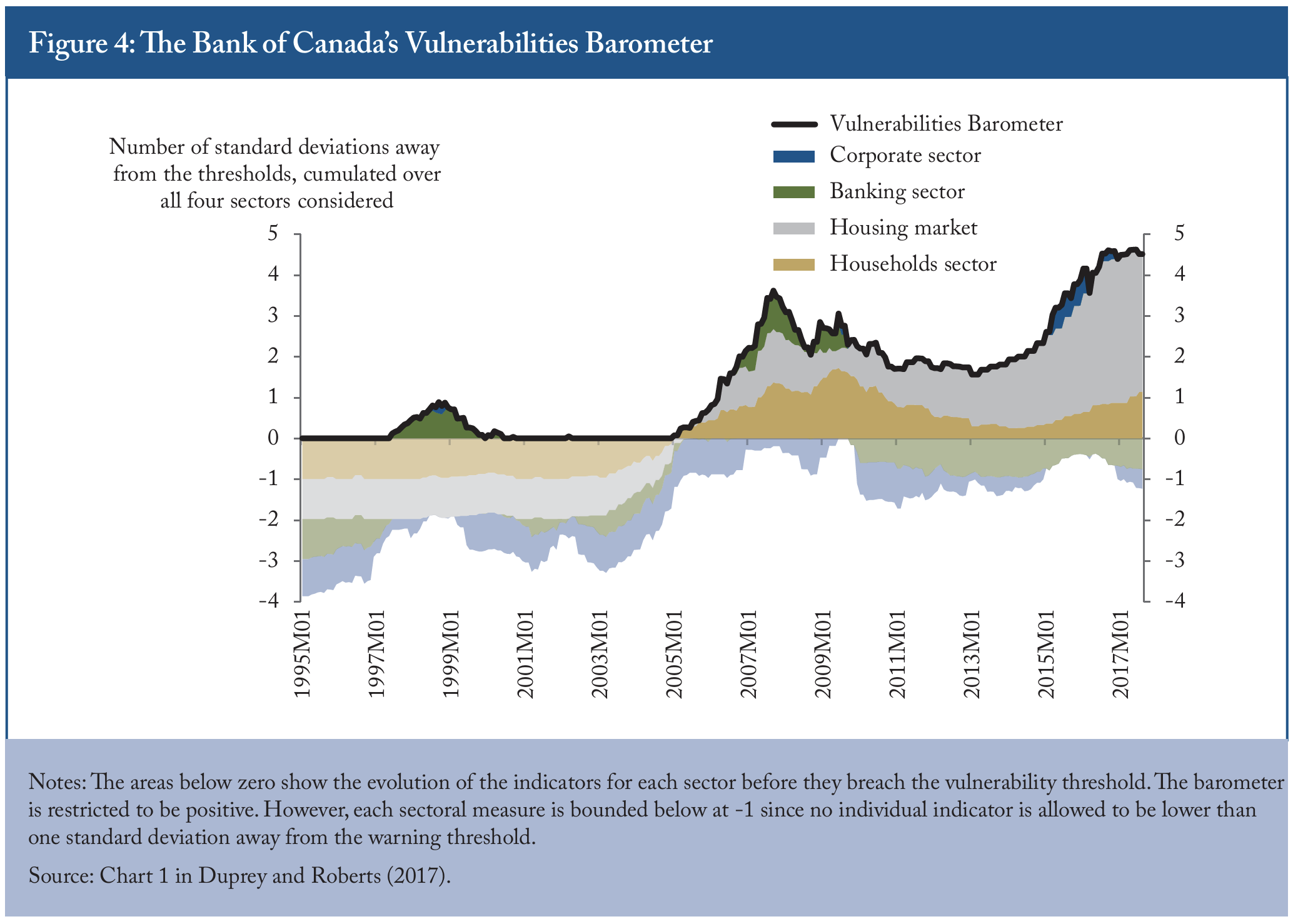
Risks at present appear to be low. This is in contrast to the Duprey and Roberts barometer, shown as Figure 4. Their barometer does capture the major crisis periods but it also results in a number of false alarms: for example, it suggests that vulnerability since 2016 has been higher than before or during the financial crisis. This explains why the Bank has frequently highlighted increasing debt in its communications. Our measure appears to mitigate some of these false positives.

Data do not exist for all variables going back to 1980, but do for some including household debt to disposable income, household debt to GDP, house price to rent ratio, and our backward-looking extension of the debt-service ratio. Our data set for the deviation of these variables from trend, therefore, stretches back to 1980. This allows us to calculate a vulnerabilities barometer with a longer life span. This longer data set encompasses two additional financial stress periods: the recession in Canada in the early 1980s and the 1987 stock market crash. As seen in Figure 5, the vulnerabilities barometer picks up these additional stress periods. The debt-service ratio provides significant value added in this earlier period. Its contribution to the vulnerabilities barometer spikes well in advance of the recession of the early 1980s and the stock market crash.¹²12 According to the C.D. Howe Institute’s Business Cycle Council, the early 1980s recession begins in June 1981 (end of the second quarter). The contribution of the debt-service ratio spikes at the beginning of our sample, the first quarter of 1980. It continues to increase well before the recession of the early 1990s, and still manages to avoid most of the false positives.

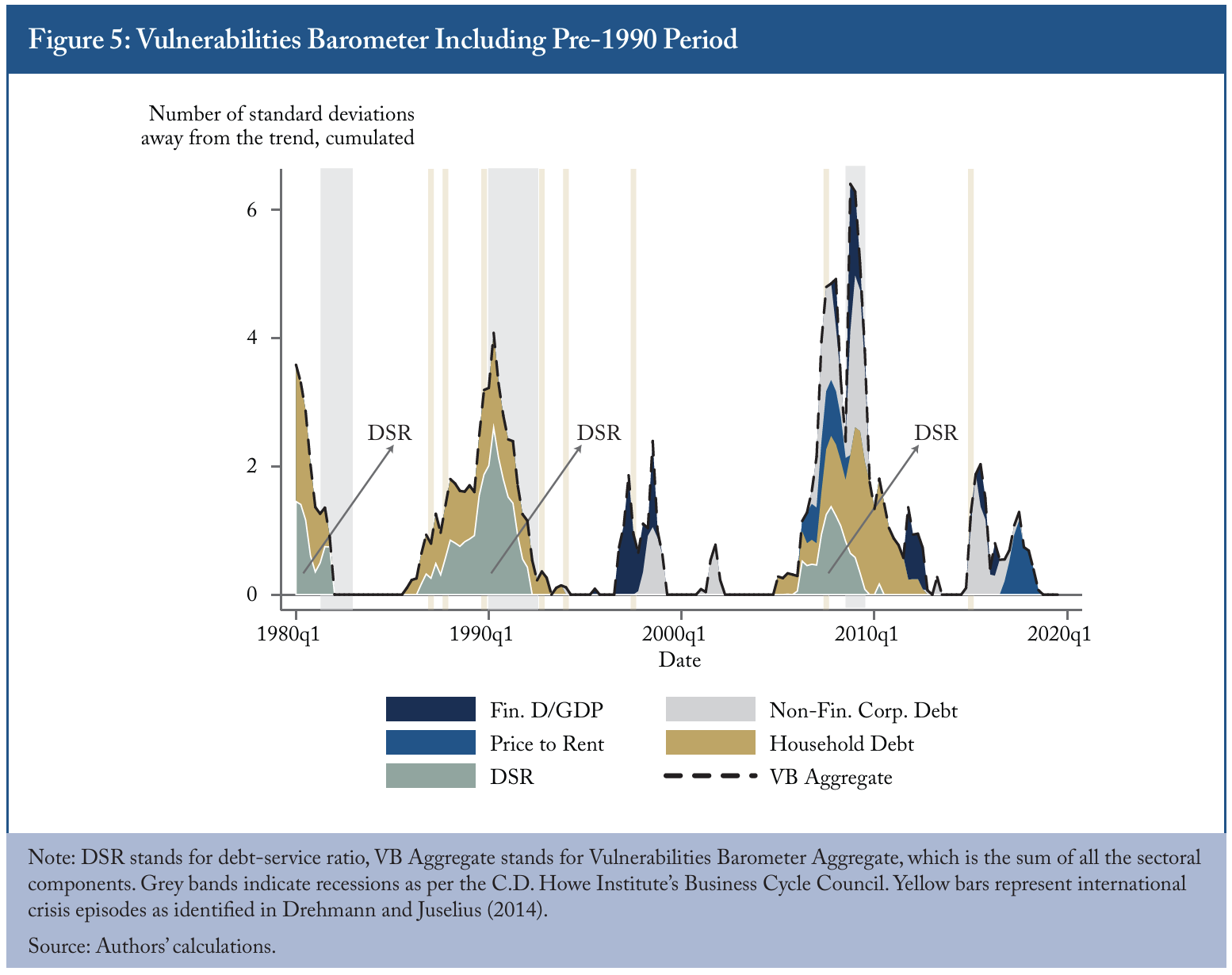
Figures 3 and 5 illustrate the potential of our vulnerabilities barometer, and in particular of debt servicing, to flag periods of financial stress and economic downturns. This leads us to examine the question of the statistical significance of debt servicing as a variable for predicting financial crises and economic slowdowns.

It makes good intuitive sense that debt servicing would be a better predictor of financial stress than debt-to-GDP/income ratios. When financial conditions change, the level of indebtedness of households and firms does not change immediately: debt will only change gradually as financial conditions affect new borrowing. However, when they eventually renew mortgages and loans (or immediately in the case of variable-interest-rate loans), they will be faced with an immediate jump in their monthly payments. If households’ saving rates and firms’ cash flows are inadequate, and if they do not have access to new sources of funding, they may find it difficult to meet their payments.

The Relationship between New Borrowing and Debt Servicing

Debt servicing is by definition linked to the dynamics of new borrowing, and helps explain why this variable played an important role in our vulnerabilities barometer.

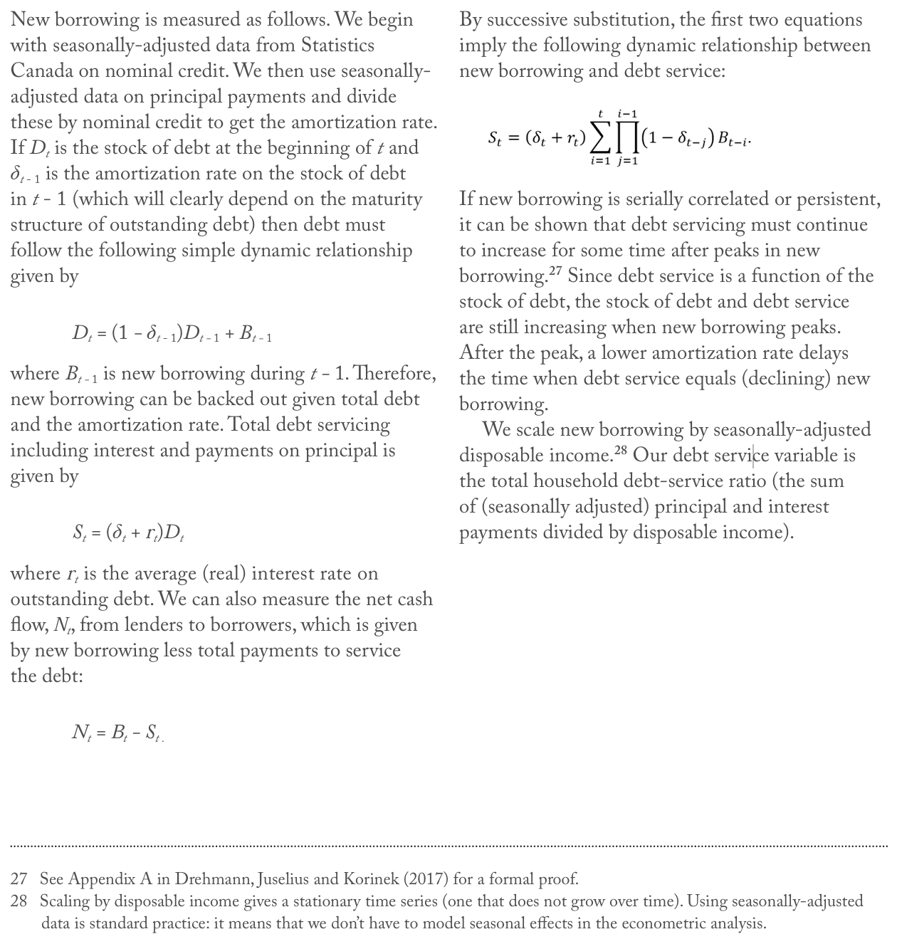
We use a simple accounting framework based on Drehmann, Juselius and Korinek (2017) to document the persistence of new borrowing and the dynamic relationship between new borrowing and debt servicing. New borrowing can be thought of as the difference between the stock of credit in the current period less the portion of the stock of credit from last period that was not paid off (more detail can be found in Appendix A). We use quarterly data from Statistics Canada on total nominal credit to construct quarterly time series for new borrowing, expressing it as a percentage of disposable income to match the denominator used in the debt-service ratio (Figure 6).

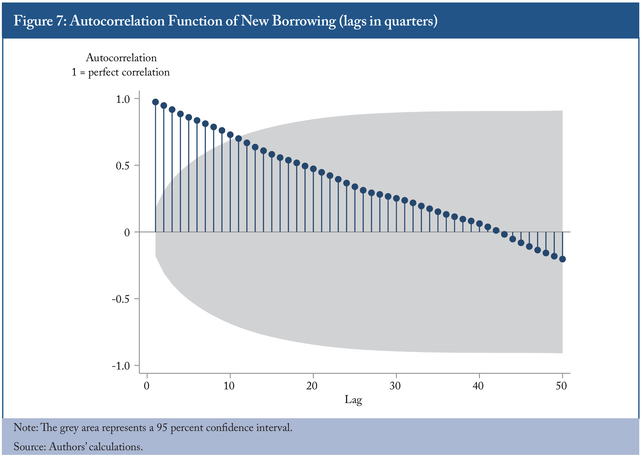
Figure 7 shows the strength of the relationship between current and past new borrowing (as measured by the autocorrelation function¹³13 The autocorrelation function measures the statistical correlation between the current value of new borrowing and its values lagged by one, two and additional periods.). New borrowing is clearly highly persistent from one quarter to the next. For example, at one lag, the correlation between new borrowing in the current period and new borrowing one quarter past is nearly one (0.98 to be exact).¹⁴14 The first-order autocorrelation coefficient of new borrowing is higher than that obtained by Drehmann, Juselius and Korinek (2017) for a cross-section of countries. This is to be expected since they use annual data while we use a quarterly data set. The grey confidence bands show that beyond 10 lags the autocorrelations are not statistically significant.

Debt servicing then follows new borrowing with a lag, as shown in Figure 8. The peak correlation between debt servicing and new borrowing occurs at a five-quarter lag. The relation between borrowing and debt servicing follows an accounting relationship, but it is not purely mechanical: variations in interest rates and amortization rates (which both depend in complex ways on the macroeconomic climate) affect the dynamic relationship between the two variables.

The Dynamic Impact of New Borrowing

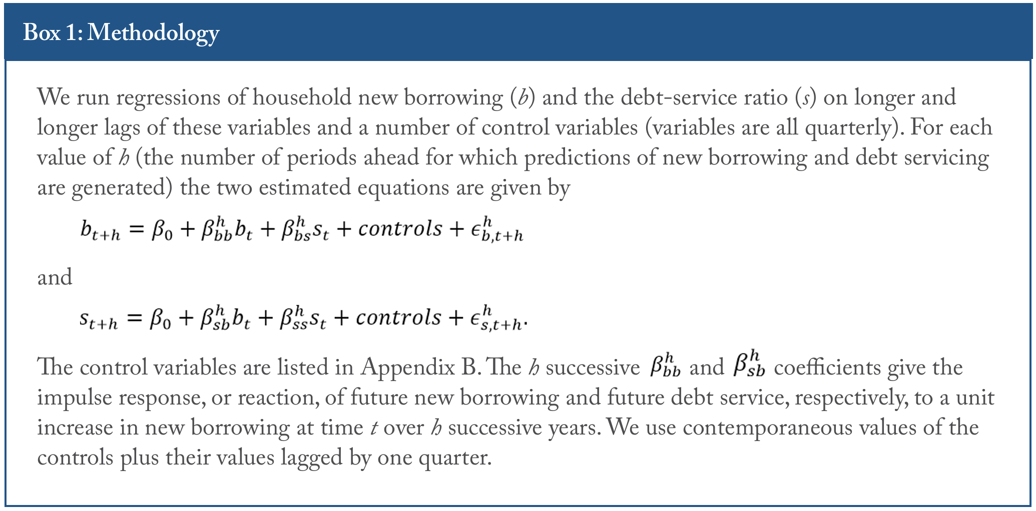
In order to provide an in-depth analysis of the relationship between household new borrowing and debt servicing, we use the local projections methodology¹⁵15 The local projections method estimates the response at each period of interest rather than extrapolating over the longer term. developed by Jorda (2005), and estimate the regressions found in Drehmann, Juselius and Korinek (2017).¹⁶16 Their study uses a sample of 17 different countries, but they are restricted to using annual data. Our data are quarterly, which adds observations in a different fashion. The first set of regressions evaluate the impact of a unit increase in new borrowing on the dynamic path of new borrowing and the debt-service ratio. The statistical methodology is described in more detail in Box 1 below.

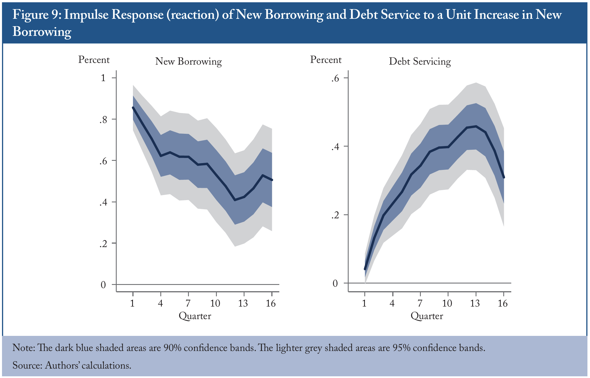
Figure 9 shows the simulated responses of new borrowing and debt service to a positive one unit change in new borrowing. The figure clearly shows that a positive shock to new borrowing persists over time and that debt servicing responds positively and with a lag. This is a clear confirmation in the data of the lag between new borrowing and the peak in debt servicing.¹⁷17 We also calculated the impulse responses of new borrowing and debt servicing to an exogenous increase in the former using an estimated structural vector autoregression with a Cholesky decomposition that allows debt servicing to respond to new borrowing only with a lag. The results were qualitatively very similar to what we find using local projections.

The Impact of New Borrowing and Debt Service on Growth and Financial Crises

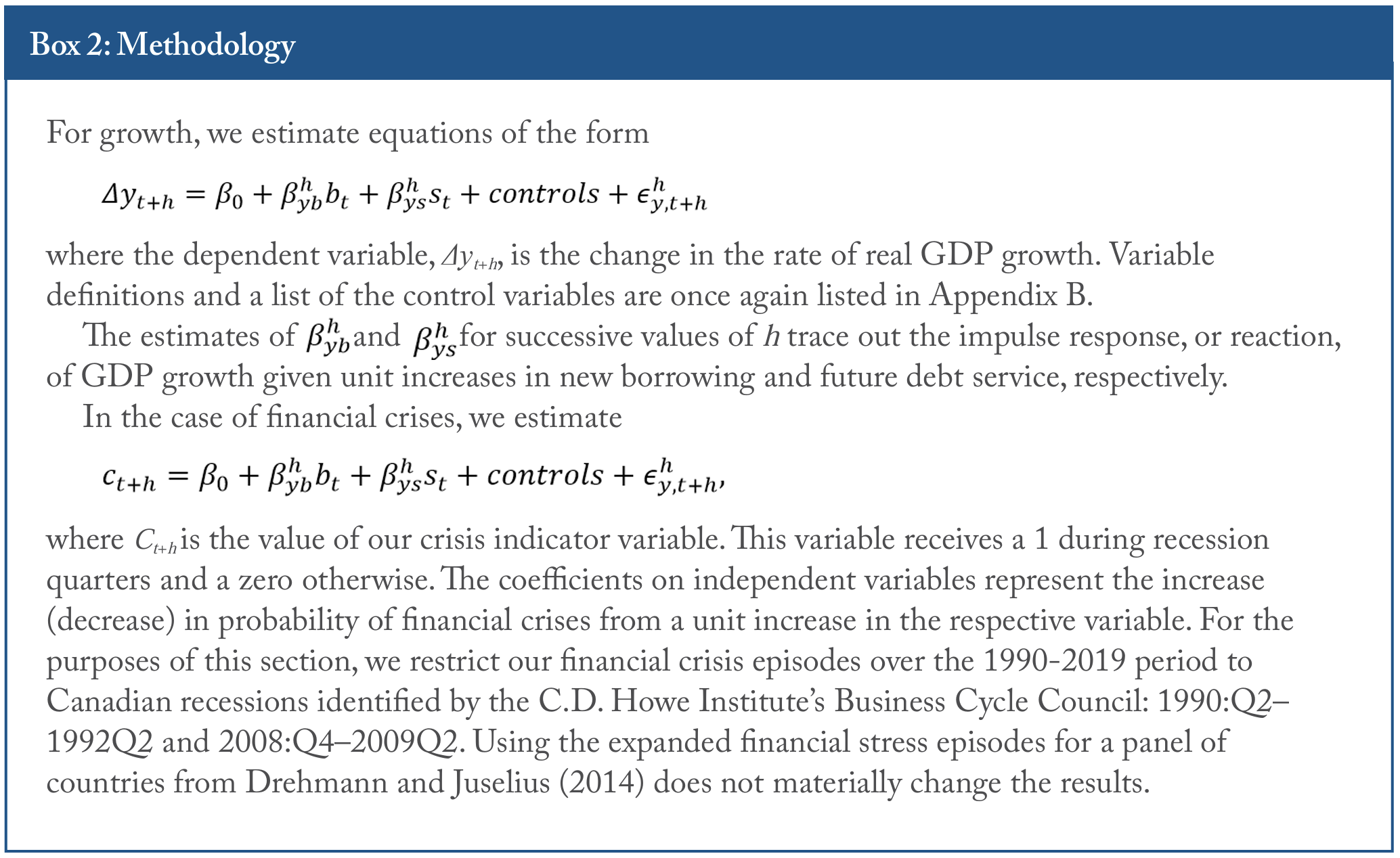
What is perhaps of more interest is the question: what are the impacts of new borrowing and debt servicing on economic growth and on financial crises? We use a similar statistical methodology, once again based on Jorda (2005), and run similar regressions to Drehmann, Juselius and Korinek (2017), to answer this question. See Box 2 for more of the technical details.

Figure 10 shows that a unit increase in new borrowing has an initial positive effect on GDP growth, but the effect turns negative in year two. An increase in debt service has an immediate negative impact on GDP growth. The negative impact of debt service on output is highly significant. What this says is that new borrowing by itself has a positive effect on GDP growth. However, this is short-lived, and when increased borrowing inevitably leads to an increase in debt servicing, the effect on GDP growth is negative.

Figure 11 shows our results for the dynamic response of the probability of financial crises to a unit increase in new borrowing and the debtservice ratio. The response of the crisis indicator variable is similar to the response of real growth, only of the opposite sign. New borrowing initially has a negative impact on the probability of financial crises, with the effect dying out in year two. An increase in new borrowing then increases the chance of financial crises, which is related to its delayed impact on debt servicing. The debt-service ratio has an immediate and pronounced positive impact on the probability of crisis, lasting out to three years.¹⁸18 Again, these results hold when we use the expanded set of financial stress episodes in the panel of countries used in Drehmann and Juselius (2014). The conclusion is, therefore, similar to the case of GDP growth: while new borrowing is initially good for the economy, it eventually leads to an increase in debt servicing, which leads to instability and increased risk of a financial crisis.¹⁹19 Our baseline local projections estimation is run using ordinary least squares. The results hold when we run a local projection using logit as well.

New Borrowing and Debt Servicing versus Debt

What happens if we run a horse race between new borrowing and debt servicing on the one hand, and more traditional measures of debt, such as creditto-GDP, on the other? We run regressions for the 1990:Q1–2019:Q3 period that are designed to forecast one-period-ahead real GDP growth and the probability of financial crises (also one-periodahead) to see which variables are more important for predicting growth and financial crises, as defined above (Tables 1 and 2).²⁰20 Regressions are run with ordinary least squares, and, in the case of financial crises, since it is a binary variable that takes on one of two possible values (zero or one), we run it with a logit regression as a robustness check. The size of the estimated coefficients change because of the logit transformation, but their sign and significance change very little compared to the ordinary least squares regression.

New borrowing and debt service are significant explanatory variables for GDP growth (Table 1). As expected, new borrowing has a positive effect on future GDP growth while the debt-service ratio has a strongly negative effect. Both variables are significant even when more traditional measures of credit are added to the regression (columns 6-9). Moreover, the magnitude of the coefficients on both new borrowing and debt service are fairly stable across different specifications. These results confirm the results in the cross-country study by Drehmann, Juselius and Korinek (2017).²¹21 They find that the impact of debt service remains stable across specifications and when different measures of debt are added. They find the new borrowing variable to be less stable, with multicollinearity affecting its estimated coefficient when different measures of debt are included. The results also remain true when we extend the forecast period of the dependent variable from one-quarter-ahead real GDP growth to one-year-ahead real GDP growth.²²22 At two years ahead, the results remain true for debt servicing, while new borrowing, despite having the same sign, loses its significance.

Credit growth also appears to be significant when included on its own, and when added to regressions that include new borrowing and the debt-service ratio. In fact, the latter has the highest percentage of variance explained (as measured by the R2) of any regression we run. The difference between credit growth and new borrowing can best be summarized with a quick example. Imagine the stock of credit this period is $100, as it was last period. Credit growth would be zero. However, if principal payments on last period’s stock were $20, and new borrowers took out $20, new borrowing would equal $20.

Year-over-year growth in credit-to-GDP, on the other hand, is insignificant when added on its own as an explanatory variable, and when added to regressions that include new borrowing and the debt-service ratio.

We also look at two different credit gap measures. Specifically, using both a one-sided and two-sided gap, where we calculate the deviation of credit-to-GDP from its trend (Gap HP1 and Gap HP2).²³23 We use a Hodrick-Prescott filter. The difference between a one-sided and two-sided gap is that in the former case we only use backward-looking data, whereas in the latter we use both backward and forward-looking data. In the case of the one-sided gap variable, it is insignificant on its own, and when added to a regression including new borrowing and debt servicing. In the case of the two-sided gap, the coefficients are significant and positive in both, though this measure is unlikely to be as useful as new borrowing and debt servicing in forecasting, since a regulator only has backward-looking information to use in assessing vulnerabilities (see Drehmann and Juselius 2014 for more details on this point).

The regression results for financial crises (Table 2) highlight even more strongly the importance of new borrowing and debt servicing. Both new borrowing and debt servicing are highly significant, and their numerical values are stable across all specifications. New borrowing significantly reduces the probability of financial crises²⁴24 Drehmann, Juselius and Korinek (2017) find a significantly positive effect in the case of new borrowing (i.e., an increase in new borrowing increases the chances of recession), though their finding is not robust to their different specifications. In fact, they find collinearity between new borrowing and the other measures, wiping away the significance of the new borrowing variable on financial crises. while the debtservice ratio has a significantly positive impact on the probability of financial crises. That is not to say that increases in new borrowing are necessarily good. As we saw earlier, eventually increases to new borrowing cause increases in the debt-service ratio, which is the measure that is cause for concern. When we extend the forecast period from one quarter ahead to one year ahead, the results remain true for debt servicing, while new borrowing, despite having the same sign, loses its significance.²⁵25 At two years ahead, the debt-service ratio loses its significance, despite maintaining the same sign.

Traditional measures, such as credit-growth and credit-to-GDP variables (ratio and the deviation from trend), however, when looked at without controlling for new borrowing and debt service, have no statistical significance. And, while their significance improves when combined with new borrowing and debt service, they have only a mild effect on the R2 when compared to the regression with just new borrowing and debt servicing as explanatory variables.

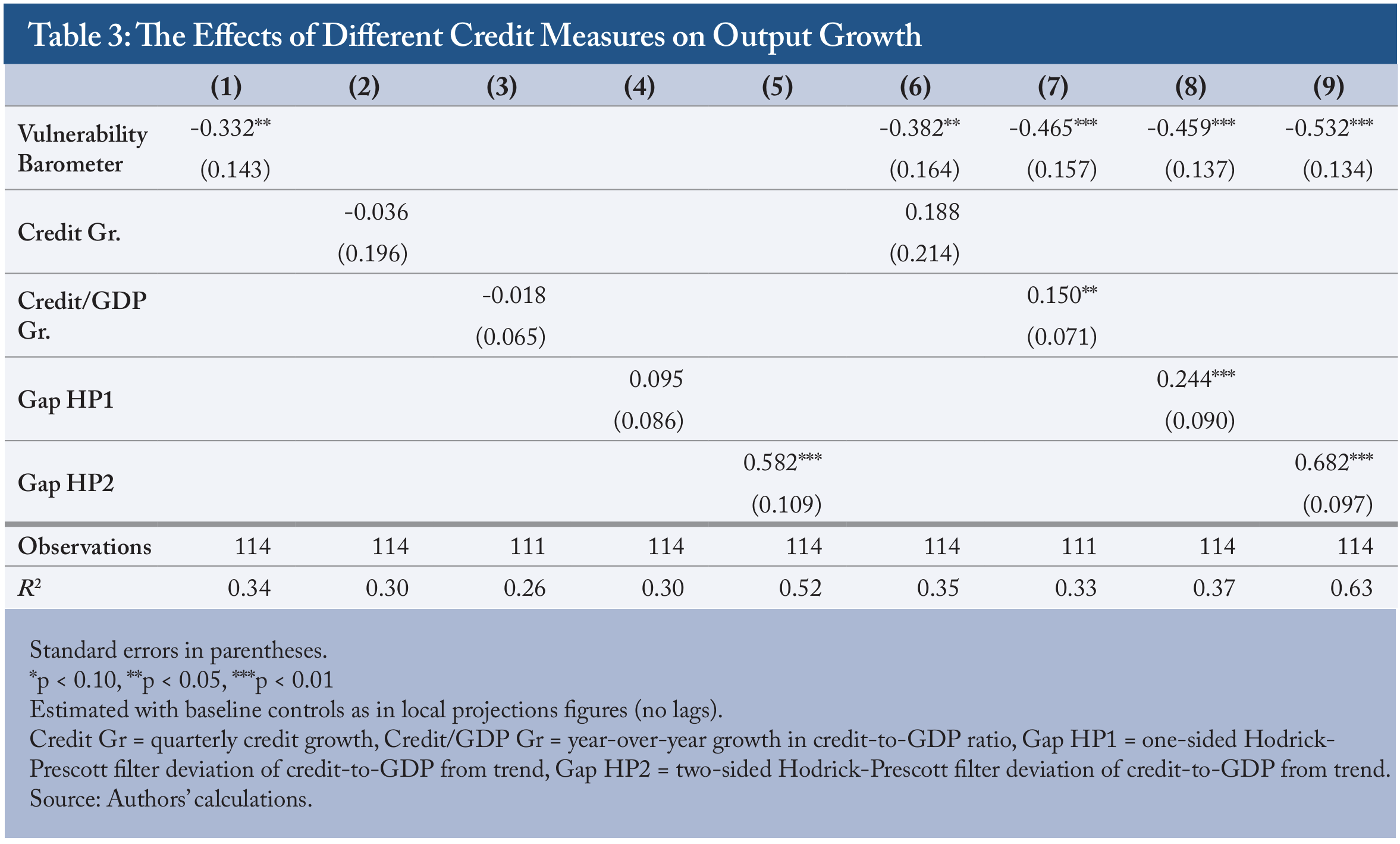
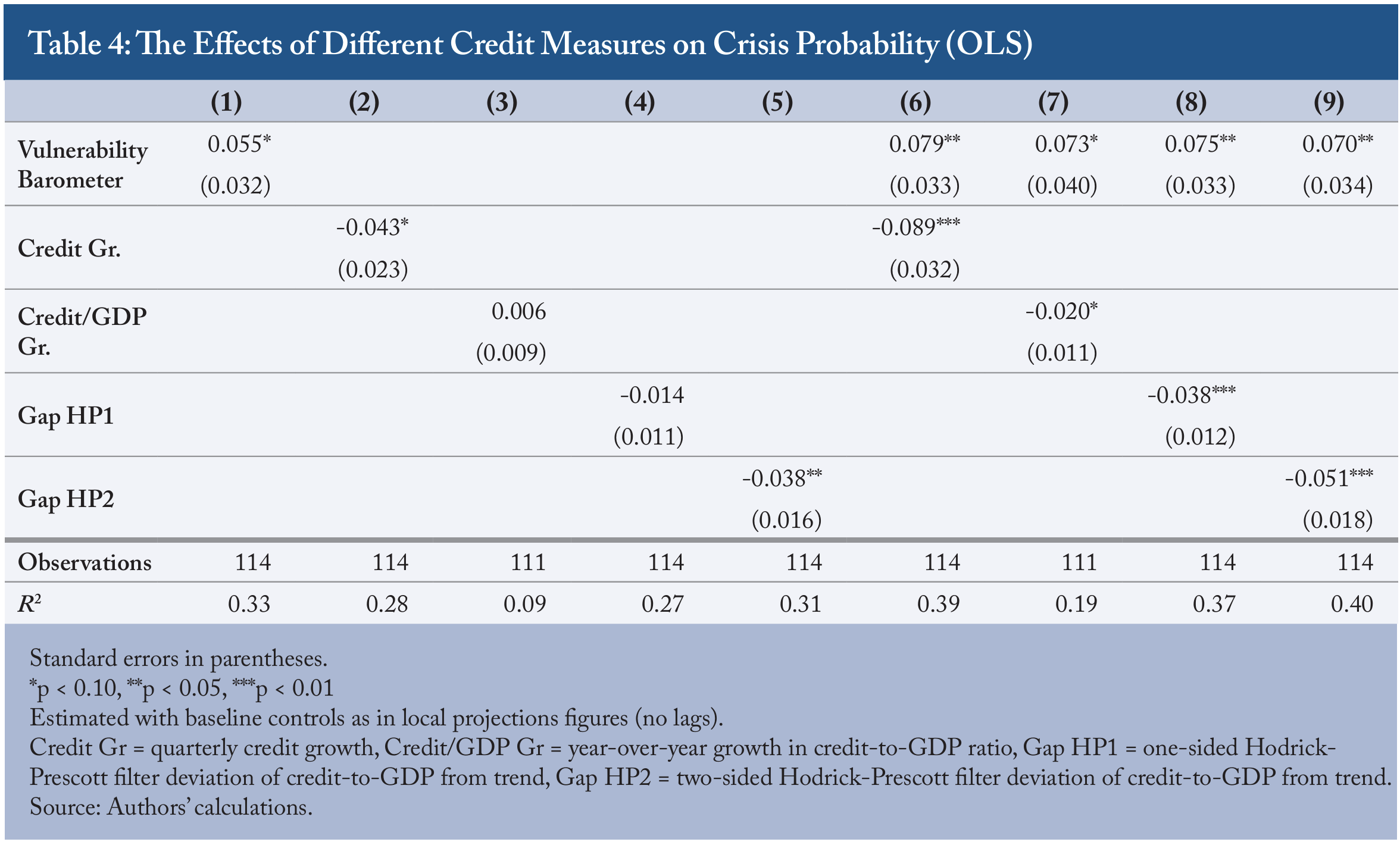
As a robustness check on our vulnerabilities barometer, and by extension the importance of the debt-service ratio, we replace new borrowing and the debt-service ratio in Tables 1 and 2 with the vulnerabilities barometer itself. We use the oneyear-ahead dependent variable, as the vulnerabilities barometer is unlikely to be of much use one quarter ahead. Table 3 indicates that the vulnerabilities barometer does a nice job of predicting a drop in economic growth. Similarly, as indicated in Table 4, it does a nice job of forecasting financial crises one year out.

Policy Discussion and Conclusion

The Canadian evidence supports the idea that the household debt-service ratio has more predictive power than debt ratios for both aggregate spending and for financial crises. Our financial vulnerability barometer provides advanced warning of crisis periods and avoids false positives, so it is a useful tool for forecasting and policy analysis.

An immediate policy conclusion is that empirical models of financial system vulnerabilities (such as Pasricha et al. 2013, Duprey and Roberts 2017 and Duprey and Ueberfeldt 2018) should put more weight on the evolution of the household debt-service ratio, and, potentially, other indicators related to debt servicing.

Further unpacking the relationship of these indicators to crises and downturns would require more granular information on debt maturity and on amortization rates. Households with different characteristics may have different propensities to borrow and consume. Households also differ in terms of the constraints they face on borrowing: when these constraints are severe, households may not be able to compensate for unexpected increases in their debt-service burdens by additional borrowing. Publicly available debt-servicing data broken down geographically would also improve the quality of related policy recommendations.

There are also policy implications for the conduct of monetary policy. If monetary policy is to take financial stability concerns into account, then central banks face a potential trade-off between the immediate effects on output and inflation and the future effects that work their way through the debt service channel.²⁶26 Of course, the dynamic impact of monetary policy will also depend on the maturity structure of debt and its distribution across households, so that our understanding of its impacts would also be improved by more granular information. Our results show this trade-off to be important.

Our analysis is for a period during which world and Canadian interest rates have trended downward. This trend explains why debt ratios in Canada have increased over time: it is rational to borrow more to purchase productive assets when the costs of borrowing are low. If interest rates were to return to the levels last seen forty years ago, this would likely also mean a long-run reduction in debt ratios. Such decreases should not be interpreted as a sign of increasing financial stability since it might also be accompanied by temporary spikes in the household debt-service ratio if interest rates increase faster than levels of debt can be reduced. Monitoring the debtservice channel would be of crucial importance in such a context. However, yield curves in developed economies show no signs of anything more than modest increases in interest rates.

Lastly, regulators concerned with the housing market and overall financial stability should look beyond traditional credit-to-GDP measures, which were always going to increase in a low interest rate environment, and closely monitor the behavior of debt servicing. This will allow a more accurate assessment of risk.

Appendix A: The Debt Servicing Series

Appendix B: Data

The variables used for new borrowing and debt service are defined in Appendix A.

The data underlying our vulnerability index are defined as follows:

1. Household debt to disposable income: monthly credit measures, turned quarterly (using monthend), divided by disposable income. Source: Statistics Canada, and authors’ calculations.
2. Housing price to rent ratio: Indexed to 100. Source: OECD.
3. Non-financial corporate debt to GDP: quarterly, market value of debt securities, loans, accounts payable. Source: Statistics Canada.
4. Financial institution debt to GDP: market value, Chartered and quasi-banks: debt securities, loans, accounts payable. Source: Statistics Canada.
5. Household debt to GDP: monthly credit measures, turned quarterly (using month-end), divided by GDP. Source: Statistics Canada, and authors’ calculations.

The independent variables in the regressions and the data sources are defined as follows.

1. GDP growth: quarterly annualized growth rate of expenditure-based real GDP, seasonally adjusted. Source: Statistics Canada.
2. Real short rate: three-month bankers’ acceptance rate minus inflation. Source: Statistics Canada and authors’ calculations.
3. Lending spread: Chartered bank prime business lending rate minus three- month bankers’ acceptance. Source: Statistics Canada and authors’ calculations.
4. Change in average lending rate on household debt: implied interest rate based on Statistics Canada household credit data and Statistics Canada interest payments (authors’ calculations).
5. Real property price growth: quarterly growth rate (authors’ calculations), where real property prices are calculated using data from the BIS.

References

Aldasoro, Iñaki, Claudio Borio, and Mathias Drehmann. 2018. “Early Warning Indicators of Banking Crises: Expanding the Family.” BIS Quarterly Review. Bank for International Settlements. March, 29–45.

Allen, Jason, Timothy Grieder, Brian Peterson, and Tom Roberts. 2017. “The Impact of Macroprudential Housing Finance Tools in Canada.” Working Paper 632, Bank for International Settlements. https://www.bis.org/publ/work632.pdf.

Ambler, Steve, Jeremy Kronick, and Farah Omran. 2019. “Household Insolvency.” Intelligence Memo. C.D. Howe Institute, April 30. https://www.cdhowe.org/intelligence-memos/ambler-kronick-omranhousehold-insolvency.

Bilyk, Olga, Alexander Ueberfeldt, and Yang Xu. 2017. “Analysis of Household Vulnerabilities Using Loan-Level Data.” Financial System Review. Bank of Canada. November, 21–33. https://www. bankofcanada.ca/wp-content/uploads/2017/11/fsrnovember2017-bilyk.pdf.

Congdon, Tim. 2017. “False Alarm.” EA Magazine. issue 9, 44–46. https://iea.org.uk/wp-content/uploads/2017/03/EA-SPRING-2017_CITYVIEW.pdf.

Drehmann, Mathias, and Mikael Juselius. 2012. “Do Debt Service Costs Affect Macroeconomic and Financial Stability?” BIS Quarterly Review. Bank for International Settlements. September, 21-36.

Drehmann, Mathias, and Mikael Juselius. 2014. “Evaluating Early Warning Indicators of Banking Crises: Satisfying Policy Requirements.” International Journal of Forecasting (30):759–780.

Drehmann, Mathias, Mikael Juselius, and Anton Korinek. 2017. “Accounting for Debt Service: The Painful Legacy of Credit Booms.” Working Paper 645, Bank for International Settlements. www. https://www.bis.org/publ/work645.pdf.

Drehmann, Mathias, and James Yetman. 2018. “Why You Should Use the Hodrick-Prescott Filter – At Least to Generate Credit Gaps.” Working Paper 744, Bank for International Settlements. www.

Duprey, Thibaut, and Tom Roberts. 2017. “A Barometer of Canadian Financial System Vulnerabilities.” Staff Analytical Note 2017-24. Ottawa: Bank of Canada. https://www.bankofcanada.ca/2017/12/staffanalytical-note-2017-24/.

Duprey, Thibaut, and Alexander Ueberfeldt. 2018. “How to Manage Macroeconomic and Financial Stability Risks: A New Framework.” Staff Analytical Note 2018-11. Ottawa: Bank of Canada. https://www.bankofcanada.ca/2018/04/staff-analyticalnote-2018-11/.

Fawcett, Tom. 2006. “An Introduction to ROC Analysis.” Pattern Recognition Letters (27): 861–874.

Flach, Peter. 2010. “ROC Analysis.” In Claude Sammut and Geoffrey Webb (eds.), Encyclopedia of Machine Learning. Boston, MA: Springer, 869–875.

Jorda, Oscar. 2005. “Estimation and inference of impulse responses by local projections.” American Economic Review (95):161–182.

Kehoe, Patrick, and Fabrizio Perri. 2002. “International Business Cycles with Endogenous Incomplete Markets.” Econometrica (70): 907–928.

Pasricha, Gurnain, Tom Roberts, Ian Christensen, and Brad Howell. 2013. “Assessing Financial System Vulnerabilities: An Early Warning Approach.” Bank of Canada Review. Autumn, 10–19.

Swets, John, Robyn Dawes, and John Monahan. 2000. “Better Decisions through Science.” Scientific American. October, 82–87.

Taylor, Alan. 2015. “Credit, Financial Stability and the Macroeconomy.” Annual Review of Economics 7, 309–339.

van Erkel, Arian, and Peter Pattynama. 1998. “Receiver Operating Characteristic (ROC) Analysis: Basic Principles and Applications in Radiology.” European Journal of Radiology (27): 88–94.